Detailed Results
We have run the implementation under Linux on a Pentium II (450MHz) PC
with 256MB memory. All test data was produced in NFF with the SPD
package (version 3.13, compiled with `JENKINS_HASH' for the scene
`mount') and was converted into binary form. No instancing was
used. Other parameters such as a screen resolution followed the
testing procedure of SPD: 513x513 eye rays were shot and the maximum
tracing depth was 5. Consult `Readme.txt' in the SPD package for more
details and scenes' properties. Parameters for refinements were
initialized as follows:
- For a bounding box hierarchy (Section 3.1):
s=3, n=1,000, and l=4 (5 levels). For `balls', `gears', and `trees', t
was set to 0.5 resulting two top-level boxes, while it was set to 1.0
for other types of scenes resulting one top-level box. The number of
resulting levels depends on types of scenes; for example, it was 3 for
`balls', while 4 to 5 for `rings'.
- For two-level grids storing rays (Section 3.2):
Ru=256 and Rl=4.
We firstly tested relatively small data (up to 50,000,000 objects/6GB)
for investigating various tendencies. Table 1 shows how refinements in Section 3.1 -
separation of geometry and bounding boxes (S), lazy
processing for each object's geometry (G), and lazy processing
with a bounding box hierarchy (B) - affect rendering (preprocess
and tracing) time. Each grid resolution was determined by the method
described in Section 3.2 and high-resolution grids were employed
if necessary. The percentage of each phase depends on both scenes and
applied refinements, but it is approximately the following: the
preprocess phase is 1-34%, the intersection phase is 49-89%, and the
shading phase is 4-37%. In this table, `SGB' becomes more effective
as data grows. Both `S' and `G' generally result in speed-up as was
expected, while the effectiveness of `B' greatly depends on the depth
complexity (how many objects a ray passes through) and/or the
occlusion complexity (how many objects are occluded) as in other
culling techniques. `B' however does not cause large overheads in
worst cases such as `tetra' and `tree'.
Table 1. Statistics for test scenes containing up to 50,000,000
objects
|
#objects |
size (MB) |
creation |
base |
SG |
SGB |
SGB/SG |
| balls6 |
597,872 |
28 |
0:00:33 |
0:05:23 |
1.11 |
1.13 |
(1.02) |
| balls7 |
5,380,841 |
251 |
0:04:45 |
0:14:18 |
1.48 |
1.57 |
(1.06) |
| balls8 |
48,427,562 |
2,263 |
0:44:50 |
1:17:16 |
1.88 |
2.00 |
(1.07) |
| gears18 |
851,473 |
107 |
0:03:09 |
0:06:12 |
1.28 |
1.34 |
(1.05) |
| gears49 |
17,176,755 |
2,167 |
1:03:28 |
0:37:36 |
1.97 |
2.40 |
(1.21) |
| gears61 |
33,139,227 |
4,181 |
2:02:32 |
1:03:58 |
1.88 |
2.57 |
(1.37) |
| gears69 |
47,962,315 |
6,051 |
2:57:17 |
1:27:21 |
1.96 |
2.90 |
(1.48) |
| mount9 |
524,292 |
49 |
0:01:08 |
0:04:53 |
1.27 |
1.34 |
(1.06) |
| mount10 |
2,097,156 |
194 |
0:04:32 |
0:10:41 |
1.64 |
1.86 |
(1.13) |
| mount11 |
8,388,612 |
776 |
0:18:06 |
0:28:45 |
2.12 |
2.67 |
(1.26) |
| mount12 |
33,554,436 |
3,104 |
1:12:11 |
1:23:15 |
2.14 |
3.06 |
(1.43) |
| rings36 |
972,361 |
86 |
0:01:29 |
0:08:46 |
1.27 |
1.51 |
(1.19) |
| rings94 |
16,877,701 |
1,499 |
0:26:21 |
1:01:11 |
1.85 |
3.07 |
(1.65) |
| rings118 |
33,279,541 |
2,955 |
0:52:10 |
1:42:10 |
1.83 |
3.62 |
(1.98) |
| rings135 |
49,755,601 |
4,418 |
1:18:12 |
2:31:03 |
1.70 |
4.48 |
(2.63) |
| teapot124 |
998,448 |
126 |
0:03:45 |
0:06:24 |
1.58 |
1.70 |
(1.08) |
| teapot516 |
17,302,512 |
2,189 |
1:05:13 |
0:52:49 |
2.22 |
2.58 |
(1.17) |
| teapot719 |
33,596,713 |
4,250 |
2:06:42 |
1:25:21 |
1.99 |
2.57 |
(1.29) |
| teapot877 |
49,986,369 |
6,323 |
3:08:32 |
1:53:10 |
2.00 |
2.58 |
(1.29) |
| tetra9 |
262,144 |
24 |
0:00:33 |
0:01:03 |
1.22 |
1.24 |
(1.02) |
| tetra10 |
1,048,576 |
97 |
0:02:13 |
0:01:52 |
1.52 |
1.60 |
(1.05) |
| tetra11 |
4,194,304 |
388 |
0:08:53 |
0:05:23 |
2.02 |
2.19 |
(1.09) |
| tetra12 |
16,777,216 |
1,552 |
0:35:32 |
0:17:37 |
2.30 |
2.53 |
(1.10) |
| tree17 |
524,287 |
47 |
0:00:42 |
0:03:53 |
1.05 |
1.04 |
(0.99) |
| tree19 |
2,097,151 |
186 |
0:02:55 |
0:05:17 |
1.14 |
1.14 |
(0.99) |
| tree21 |
8,388,607 |
744 |
0:11:42 |
0:09:44 |
1.31 |
1.31 |
(1.00) |
| tree23 |
33,554,431 |
2,880 |
0:46:30 |
0:25:12 |
1.38 |
1.39 |
(1.00) |
|
where `creation' shows time for both executing a SPD command and
converting its NFF output into binary form, and `base' shows rendering
time without refinements. Time is shown in
hours:minutes:seconds. Values in the next two columns show gain
factors for `base' (thus dividing `base' time by the gain factor gets
absolute time). `S' means separation of geometry and bounding
boxes, `G' means lazy processing for each object's
geometry, and `B' means lazy processing with a bounding box
hierarchy. `SGB' includes time for creating a bounding box
hierarchy. The values in parentheses show `SGB' to `SG' gain factors.
|
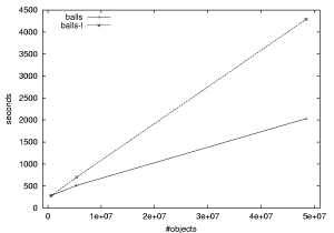
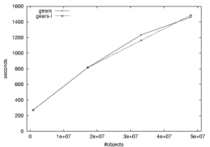
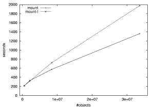
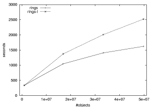
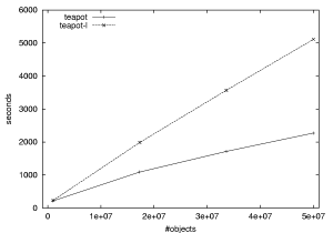
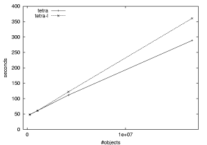
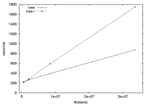
Figure 1 and Table 2 show how refinements in Section 3.2 are
efficient in realizing high-resolution grids. In the figure, slow
growth of time is achieved with refinements, while limited-resolution
grids result in more linear growth of time. Although shorter absolute
time is achieved with limited-resolution grids in `gears', it changes
linearly for latter three size factors. The table shows overheads of
two-level grids. There is 10-20% loss, which is rewarded with the
efficiency of high-resolution grids.
Table 2. Overheads of two-level grids
|
64/2 |
32/4 |
| balls8 |
0.89 |
0.90 |
| gears69 |
0.90 |
0.86 |
| mount12 |
0.81 |
0.86 |
| rings135 |
0.93 |
0.83 |
| teapot877 |
0.89 |
0.92 |
| tetra12 |
0.84 |
0.77 |
| tree23 |
0.93 |
0.91 |
|
where those values show gain factors, in comparison with single-level
grids whose maximum resolution is limited to 128. `64/2' and `32/4'
mean two-level grids whose maximum upper/lower resolutions are 64/2
and 32/4 respectively.
|
The next results show how refinements are efficient for huge data.
Table 3 and Table 4 show statistics and Figure 2 shows their rendered images. These tables
show that applying refinements for huge data further improves both
preprocess and tracing time. The gain factors range from 5 to 14 in
rendering time. The gain factor in tracing time is quite large for
`rings368m' (`rings368' with different view data), because only a
small portion of objects contributed to the image and many objects
were culled by `B'. Note that it is not an ordinary view-frustum
culling; there are reflection/shadow rays going outside the
frustum. Note also that high-resolution grids were used by applying
refinements in Section 3.2 even for `base', as in Table 1, in order to avoid lengthy computation
time. The gain factors would be much larger if the grid resolution for
`base' was limited.
Creation time is extremely long for large data. This results from
strictly following the testing procedure of SPD. In actual systems,
however, it is important to cooperate with modeling systems for
efficient rendering of huge data.
Table 3. Statistics for huge data (total)
|
#objects |
size (MB) |
creation |
base |
SG |
SGB |
SGB/SG |
| mount14 |
536,870,916 |
49,664 |
19:16:15 |
19:26:15 |
2.04 |
5.33 |
(2.62) |
| rings368 |
1,000,787,041 |
88,857 |
26:37:42 |
50:54:40 |
1.84 |
12.43 |
(6.76) |
| rings368m |
1,000,787,041 |
88,857 |
26:37:42 |
30:40:26 |
1.65 |
13.65 |
(8.26) |
|
where data is shown in the same format of Table 1. The view parameter is the only difference
between `rings368m' and `rings368': the view frustum of `rings368m'
contains approximately 1,000,000 objects.
|
Table 4. Statistics for huge data (preprocess/tracing)
|
preprocess |
tracing |
|
base |
SG |
SGB |
SGB/SG |
base |
SG |
SGB |
SGB/SG |
| mount14 |
6:31:37 |
2.10 |
8.87 |
(4.23) |
12:54:37 |
2.01 |
4.44 |
(2.21) |
| rings368 |
11:03:30 |
1.82 |
5.61 |
(3.09) |
39:51:10 |
1.84 |
18.76 |
(10.17) |
| rings368m |
11:03:30 |
1.82 |
5.61 |
(3.09) |
19:36:56 |
1.57 |
70.78 |
(45.01) |
|
where data is shown in the same format of Table 3.
|
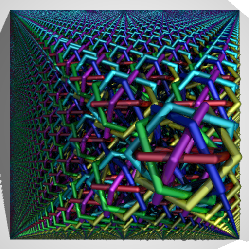
Figure 2. Rendered images for huge data. The view parameter is the
only difference between `rings368m' and `rings368': the view frustum
of `rings368m' contains approximately 1,000,000 objects.
 |
 |
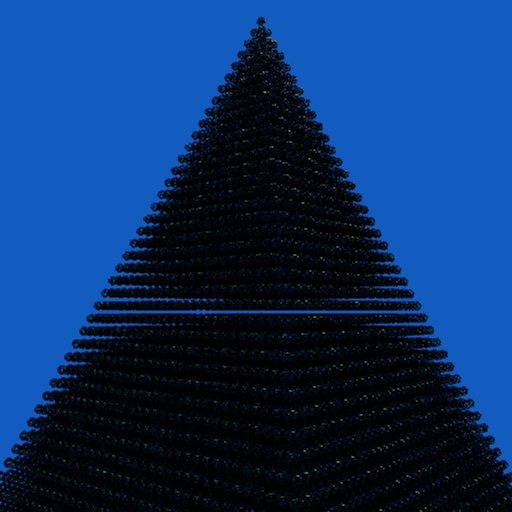 |
| mount14 |
rings368 |
rings368m |
| #objects: 536,870,916 |
#objects: 1,000,787,041 |
#objects: 1,000,787,041 |
| 48.50GB |
86.77GB |
86.77GB |